Page 276 - Intelligent Digital Oil And Gas Fields

226 Intelligent Digital Oil and Gas Fields

during the entire life span of the well or completion event (e.g., depletion
period and artificial lift completion). The simulator can run quickly but
may sacrifice some accuracy related to production rate changes.
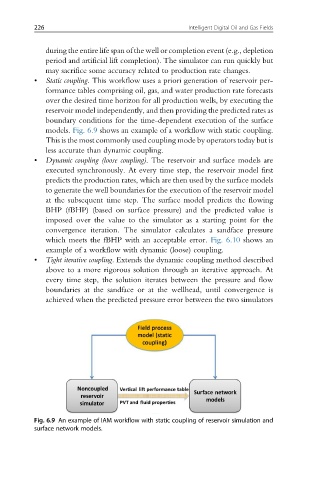
• Static coupling. This workflow uses a priori generation of reservoir per-
formance tables comprising oil, gas, and water production rate forecasts
over the desired time horizon for all production wells, by executing the
reservoir model independently, and then providing the predicted rates as
boundary conditions for the time-dependent execution of the surface
models. Fig. 6.9 shows an example of a workflow with static coupling.
This is the most commonly used coupling mode by operators today but is
less accurate than dynamic coupling.
• Dynamic coupling (loose coupling). The reservoir and surface models are
executed synchronously. At every time step, the reservoir model first
predicts the production rates, which are then used by the surface models
to generate the well boundaries for the execution of the reservoir model
at the subsequent time step. The surface model predicts the flowing
BHP (fBHP) (based on surface pressure) and the predicted value is
imposed over the value to the simulator as a starting point for the
convergence iteration. The simulator calculates a sandface pressure
which meets the fBHP with an acceptable error. Fig. 6.10 shows an
example of a workflow with dynamic (loose) coupling.
• Tight iterative coupling. Extends the dynamic coupling method described
above to a more rigorous solution through an iterative approach. At
every time step, the solution iterates between the pressure and flow
boundaries at the sandface or at the wellhead, until convergence is
achieved when the predicted pressure error between the two simulators

Fig. 6.9 An example of IAM workflow with static coupling of reservoir simulation and
surface network models.