Page 277 - Intelligent Digital Oil And Gas Fields

Integrated Asset Management and Optimization Workflows 227

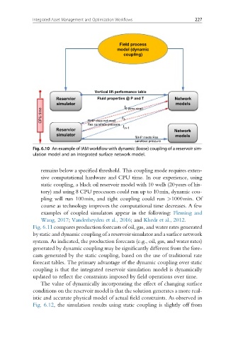
Field process
model (dynamic
coupling)

Vertical lift performance table
Reservior Fluid properties @ P and T Network
simulator t 0 (time step) models
CPU time t 1
fBHP does not meet
Res sandface pressure
t
Reservior n+1 Network
simulator models
fBHP meets Res
sandface pressure
Fig. 6.10 An example of IAM workflow with dynamic (loose) coupling of a reservoir sim-
ulation model and an integrated surface network model.

remains below a specified threshold. This coupling mode requires exten-
sive computational hardware and CPU time. In our experience, using
static coupling, a black oil reservoir model with 10 wells (20years of his-
tory) and using 8 CPU processors could run up to 10min, dynamic cou-
pling will run 100min, and tight coupling could run >1000min. Of
course as technology improves the computational time decreases. A few
examples of coupled simulators appear in the following: Fleming and
Wang, 2017; Vanderheyden et al., 2016;and Khedr et al., 2012.
Fig. 6.11 compares production forecasts of oil, gas, and water rates generated
by static and dynamic coupling of a reservoir simulator and a surface network
system. As indicated, the production forecasts (e.g., oil, gas, and water rates)
generated by dynamic coupling may be significantly different from the fore-
casts generated by the static coupling, based on the use of traditional rate
forecast tables. The primary advantage of the dynamic coupling over static
coupling is that the integrated reservoir simulation model is dynamically
updated to reflect the constraints imposed by field operations over time.
The value of dynamically incorporating the effect of changing surface
conditions on the reservoir model is that the solution generates a more real-
istic and accurate physical model of actual field constraints. As observed in
Fig. 6.12, the simulation results using static coupling is slightly off from