Page 168 - Intermediate Statistics for Dummies

12_045206 ch07.qxd 2/1/07 9:56 AM Page 147
Chapter 7: When Data Throws You a Curve: Using Nonlinear Regression
If you look at the section “Assessing the fit of a polynomial model,” you can
figure out how to apply these assessment strategies to the straight-line fit
of log(y).
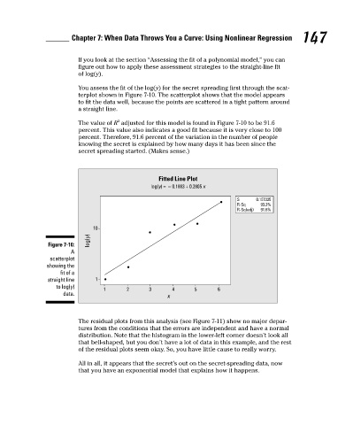
You assess the fit of the log(y) for the secret spreading first through the scat-
terplot shown in Figure 7-10. The scatterplot shows that the model appears
to fit the data well, because the points are scattered in a tight pattern around
a straight line.
2
The value of R adjusted for this model is found in Figure 7-10 to be 91.6
percent. This value also indicates a good fit because it is very close to 100
percent. Therefore, 91.6 percent of the variation in the number of people
knowing the secret is explained by how many days it has been since the
secret spreading started. (Makes sense.)
Fitted Line Plot 147
log(y) = − 0.1883 + 0.2805 x
S 0.157335
R-Sq 93.3%
R-Sq(adj) 91.6%
10
log(y)
Figure 7-10:
A
scatterplot
showing the
fit of a
straight line 1
to log(y)
1 2 3 4 5 6
data.
x
The residual plots from this analysis (see Figure 7-11) show no major depar-
tures from the conditions that the errors are independent and have a normal
distribution. Note that the histogram in the lower-left corner doesn’t look all
that bell-shaped, but you don’t have a lot of data in this example, and the rest
of the residual plots seem okay. So, you have little cause to really worry.
All in all, it appears that the secret’s out on the secret-spreading data, now
that you have an exponential model that explains how it happens.