Page 167 - Intermediate Statistics for Dummies

12_045206 ch07.qxd 2/1/07 9:56 AM Page 146
146
Part II: Making Predictions by Using Regression
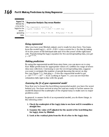
Figure 7-9:
Regression Analysis: Day versus Number
Minitab fits
a line to the
The regression equation is
log(y) for the
logten (number) = − 0.1883 + 0.2805 day
secret-
S = 0.157335
spreading
R−Sq = 93.3%
data.
Going exponential
After you have your Minitab output, you’re ready for step three. You trans-
form the model log(y) = –0.19 + 0.28 x into a model for y. Do this by taking
*
10 to the power of the left-hand side and 10 to the power of the right-hand
side. Transforming the log(y) equation for the secret-spreading data, you get
–0.19+0.28x
.
y = 10
Making predictions R−Sq(adj) = 91.6%
By using the exponential model from step three, you can move on to step
four: Make predictions for appropriate values of x (within the range of where
data was collected). Continuing to use the secret-spreading data, suppose
you want to estimate the number of people knowing the secret on day
five (see Figure 7-1). Just plug x = 5 into the exponential model to get
* = 10
y = 10 –0.19+0.28 5 1.21 = 16.22. Looking at Figure 7-1, you can see that this
estimation falls right in line with the graph.
Assessing the fit of your exponential model
Now that you’ve found the best-fitting exponential model, you have the worst
behind you. You have arrived at step five and are ready to further assess the
model fit (beyond the scatterplot of the original data) to make sure no major
problems arise.
In general, to assess the fit of an exponential model, you do three things, in
the following order:
1. Check the scatterplot of the log(y) data to see how well it resembles a
straight line.
2
2. Examine the value of R adjusted for the model of the best-fitting line
for log(y), done by Minitab.
3. Look at the residual plots from the fit of a line to the log(y) data.