Page 95 - Intermediate Statistics for Dummies

09_045206 ch04.qxd 2/1/07 9:49 AM Page 74
74
Part II: Making Predictions by Using Regression
Finding the best-fitting line
to model your data
After you’ve established that x and y have a strong linear relationship, as evi-
denced by both the scatterplot and the correlation coefficient (see the previ-
ous sections), you’re ready to build a model that estimates y using x. In the
textbook-weight case, you want to estimate average textbook weight using
average student weight.
The most basic of all the regression models is the simple linear regression
model that comes in the general form of y = a + bx. Here a represents the y-
intercept of the line; b represents the slope.
A straight line that’s used in simple linear regression is just one of an entire
family of models (or functions) that statisticians use to express relationships
between variables. A model is just a general name for a function that you can
use to estimate or guess what outcome will occur if you have some given
information about related items.
To find the right model for your data, the idea is to scour all possible lines and
choose the one that fits the data best. Thankfully, you have an algorithm that
does this for you (computers use it in their calculations). Formulas also exist
for finding the slope and y-intercept of the best-fitting line by hand. (You can
find those formulas in your intro stats text or in Statistics For Dummies [Wiley].)
To run a linear regression analysis in Minitab, go to Stat>Regression>
Regression. Highlight the response (y) variable in the left-hand box, and click
on Select. The variable shows up in the Response Variable box. Then high-
light your explanatory (x) variable, and click on Select. This variable shows
up in the Predictor Variable box. Click OK.
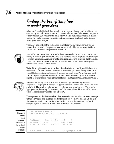
The equation of the line that best describes the relationship between average
textbook weight and average student weight is: y = 3.69 + 0.113x, where x is
the average student weight for that grade, and y is the average textbook
weight. Figure 4-2 shows the Minitab output of this analysis.
The regression equation is
Figure 4-2: textbook wt = 3.69 + 0.113 student wt
Simple
linear
regression Predictor Coef SE Coef T P
analysis for Constant 3.694 1.395 2.65 0.024
student wt 0.11337 0.01456 7.78 0.000
the textbook
weight
example.
S = 1.51341 R-Sq = 85.8% R-Sq(adj) = 84.4%