Page 292 - Intro to Tensor Calculus

286

∗
∗
where λ ,µ and ν are constants. Examining the results from equations (2.5.11) and (2.5.13) we find that if
∗
the viscous stress is symmetric, then τ ij = τ ji . This requires ν be chosen as zero. Consequently, the viscous
∗
stress tensor reduces to the form
τ ik = λ δ ik v p,p + µ (v k,i + v i,k ). (2.5.17)
∗
∗
∗
∗
The coefficient µ is called the first coefficient of viscosity and the coefficient λ is called the second coefficient
of viscosity. Sometimes it is convenient to define
2
∗
ζ = λ + µ ∗ (2.5.18)
3
as “another second coefficient of viscosity,” or “bulk coefficient of viscosity.” The condition of zero bulk
viscosity is known as Stokes hypothesis. Many fluids problems assume the Stoke’s hypothesis. This requires
that the bulk coefficient be zero or very small. Under these circumstances the second coefficient of viscosity
2
is related to the first coefficient of viscosity by the relation λ = − µ . In the study of shock waves and
∗
∗
3
acoustic waves the Stoke’s hypothesis is not applicable.
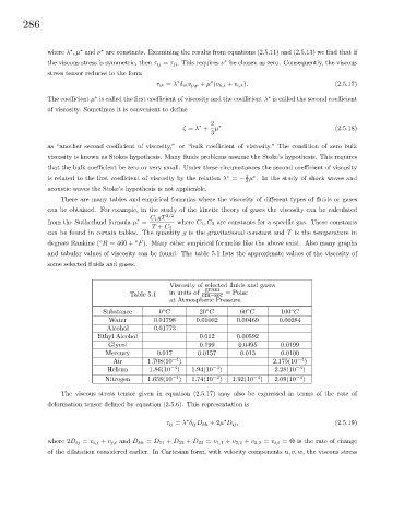
There are many tables and empirical formulas where the viscosity of different types of fluids or gases
can be obtained. For example, in the study of the kinetic theory of gases the viscosity can be calculated
C 1 gT 3/2
∗
from the Sutherland formula µ = where C 1 ,C 2 are constants for a specific gas. These constants
T + C 2
can be found in certain tables. The quantity g is the gravitational constant and T is the temperature in
o
o
degrees Rankine ( R = 460 + F). Many other empirical formulas like the above exist. Also many graphs
and tabular values of viscosity can be found. The table 5.1 lists the approximate values of the viscosity of
some selected fluids and gases.

Viscosity of selected fluids and gases
gram
Table 5.1 in units of cm−sec =Poise
at Atmospheric Pressure.
Substance 0 C 20 C 60 C 100 C
◦
◦
◦
◦
Water 0.01798 0.01002 0.00469 0.00284
Alcohol 0.01773
Ethyl Alcohol 0.012 0.00592
Glycol 0.199 0.0495 0.0199
Mercury 0.017 0.0157 0.013 0.0100
Air 1.708(10 −4 ) 2.175(10 −4 )
Helium 1.86(10 −4 ) 1.94(10 −4 ) 2.28(10 −4 )
Nitrogen 1.658(10 −4 ) 1.74(10 −4 ) 1.92(10 −4 ) 2.09(10 −4 )

The viscous stress tensor given in equation (2.5.17) may also be expressed in terms of the rate of
deformation tensor defined by equation (2.5.6). This representation is

∗
∗
τ ij = λ δ ij D kk +2µ D ij , (2.5.19)
where 2D ij = v i,j + v j,i and D kk = D 11 + D 22 + D 33 = v 1,1 + v 2,2 + v 3,3 = v i,i = Θ is the rate of change
of the dilatation considered earlier. In Cartesian form, with velocity components u, v, w, the viscous stress