Page 20 -

1. Setting the Scene
6

u 0 =1 +
1
10
u 0 =1

t
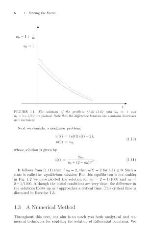
FIGURE 1.1. The solution of the problem (1.5)–(1.6) with u 0 =1 and
u 0 = 1+1/10 are plotted. Note that the difference between the solutions decreases
as t increases.
Next we consider a nonlinear problem;

u (t)= tu(t)(u(t) − 2),
(1.10)
u(0) = u 0 ,
whose solution is given by

u(t)= 2u 0 . (1.11)
u 0 +(2 − u 0 )e t 2
It follows from (1.11) that if u 0 = 2, then u(t) = 2 for all t ≥ 0. Such a
state is called an equilibrium solution. But this equilibrium is not stable;
in Fig. 1.2 we have plotted the solution for u 0 =2 − 1/1000 and u 0 =
2+1/1000. Although the initial conditions are very close, the difference in
the solutions blows up as t approaches a critical time. This critical time is
discussed in Exercise 1.3.

1.3 A Numerical Method

Throughout this text, our aim is to teach you both analytical and nu-
merical techniques for studying the solution of differential equations. We