Page 23 -

3
3
2.5
∆t =1/6
2
2
1.5
1.5
1
1
0.5
3
3
2.5
2.5
∆t =1/24
∆t =1/12
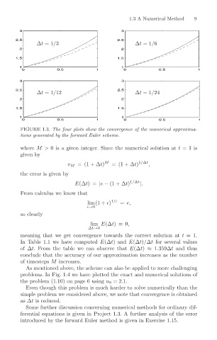
2 0 ∆t =1/3 0.5 1 2.5 0 1.3 A Numerical Method 9 1
2
1.5 1.5
1 1
0 0.5 1 0 0.5 1
FIGURE 1.3. The four plots show the convergence of the numerical approxima-
tions generated by the forward Euler scheme.
where M> 0 is a given integer. Since the numerical solution at t =1 is
given by
v M = (1+∆t) M = (1+∆t) 1/∆t ,
the error is given by
E(∆t)= |e − (1+∆t) 1/∆t |.
From calculus we know that
lim(1 + ) 1/ = e,
→0
so clearly
lim E(∆t)=0,
∆t→0
meaning that we get convergence towards the correct solution at t =1.
In Table 1.1 we have computed E(∆t) and E(∆t)/∆t for several values
of ∆t. From the table we can observe that E(∆t) ≈ 1.359∆t and thus
conclude that the accuracy of our approximation increases as the number
of timesteps M increases.
As mentioned above, the scheme can also be applied to more challenging
problems. In Fig. 1.4 we have plotted the exact and numerical solutions of
the problem (1.10) on page 6 using u 0 =2.1.
Even though this problem is much harder to solve numerically than the
simple problem we considered above, we note that convergence is obtained
as ∆t is reduced.
Some further discussion concerning numerical methods for ordinary dif-
ferential equations is given in Project 1.3. A further analysis of the error
introduced by the forward Euler method is given in Exercise 1.15.