Page 24 -

1. Setting the Scene
10
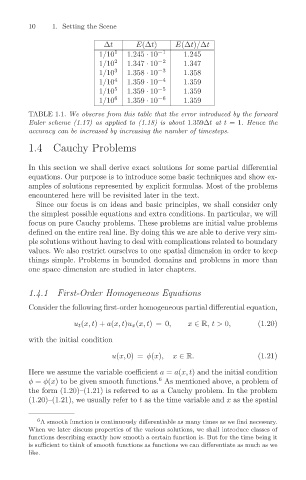
∆t
1/10
1.245
1.245 · 10
1
1.347 · 10
1/10
1.347
−2
2
1.358
1/10
1.358 · 10
−3
3
1.359
1/10
1.359 · 10
4
−4
1/10
1.359
1.359 · 10
5
−5
1.359
1/10
1.359 · 10
6
−6
TABLE 1.1. We observe from this table that the error introduced by the forward
Euler scheme (1.17) as applied to (1.18) is about 1.359∆t at t =1. Hence the
accuracy can be increased by increasing the number of timesteps.
1.4 Cauchy Problems E(∆t) −1 E(∆t)/∆t
In this section we shall derive exact solutions for some partial differential
equations. Our purpose is to introduce some basic techniques and show ex-
amples of solutions represented by explicit formulas. Most of the problems
encountered here will be revisited later in the text.
Since our focus is on ideas and basic principles, we shall consider only
the simplest possible equations and extra conditions. In particular, we will
focus on pure Cauchy problems. These problems are initial value problems
defined on the entire real line. By doing this we are able to derive very sim-
ple solutions without having to deal with complications related to boundary
values. We also restrict ourselves to one spatial dimension in order to keep
things simple. Problems in bounded domains and problems in more than
one space dimension are studied in later chapters.
1.4.1 First-Order Homogeneous Equations
Consider the following first-order homogeneous partial differential equation,
u t (x, t)+ a(x, t)u x (x, t)=0, x ∈ R,t > 0, (1.20)
with the initial condition
u(x, 0) = φ(x), x ∈ R. (1.21)
Here we assume the variable coefficient a = a(x, t) and the initial condition
φ = φ(x) to be given smooth functions. As mentioned above, a problem of
6
the form (1.20)–(1.21) is referred to as a Cauchy problem. In the problem
(1.20)–(1.21), we usually refer to t as the time variable and x as the spatial
6
A smooth function is continuously differentiable as many times as we find necessary.
When we later discuss properties of the various solutions, we shall introduce classes of
functions describing exactly how smooth a certain function is. But for the time being it
is sufficient to think of smooth functions as functions we can differentiate as much as we
like.