Page 21 -

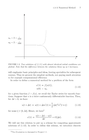
u 0 =2 +
1
1000 1.3 A Numerical Method 7
u 0 =2 − 1
1000

t

FIGURE 1.2. Two solutions of (1.11) with almost identical initial conditions are
plotted. Note that the difference between the solutions blows up as t increases.

will emphasize basic principles and ideas, leaving specialties for subsequent
courses. Thus we present the simplest methods, not paying much attention
to for example computational efficiency.
In order to define a numerical method for a problem of the form

u (t)= f u(t) ,
(1.12)
u(0) = u 0 ,
for a given function f = f(u), we recall the Taylor series for smooth func-
tions. Suppose that u is a twice continuously differentiable function. Then,
for ∆t> 0, we have
1

2
u(t +∆t)= u(t)+∆tu (t)+ (∆t) u (t + ξ) (1.13)
2
for some ξ ∈ [0, ∆t]. Hence, we have 5
u(t +∆t) − u(t)
u (t)= + O ∆t . (1.14)

∆t
We will use this relation to put up a scheme for computing approximate
solutions of (1.12). In order to define this scheme, we introduce discrete

5 The O-notation is discussed in Project 1.1.