Page 149 - Introduction to AI Robotics

132
4 The Reactive Paradigm

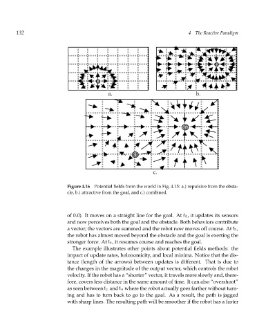
Figure 4.16 Potential fields from the world in Fig. 4.15: a.) repulsive from the obsta-
cle, b.) attractive from the goal, and c.) combined.

of 0.0). It moves on a straight line for the goal. At t 2 , it updates its sensors
and now perceives both the goal and the obstacle. Both behaviors contribute
a vector; the vectors are summed and the robot now moves off course. At t 3 ,
the robot has almost moved beyond the obstacle and the goal is exerting the
stronger force. At t 4 , it resumes course and reaches the goal.
The example illustrates other points about potential fields methods: the
impact of update rates, holonomicity, and local minima. Notice that the dis-
tance (length of the arrows) between updates is different. That is due to
the changes in the magnitude of the output vector, which controls the robot
velocity. If the robot has a “shorter” vector, it travels more slowly and, there-
fore, covers less distance in the same amount of time. It can also “overshoot”
as seen between t 3 and t 4 where the robot actually goes farther without turn-
ing and has to turn back to go to the goal. As a result, the path is jagged
with sharp lines. The resulting path will be smoother if the robot has a faster