Page 150 - Introduction to AI Robotics

4.4 Potential Fields Methodologies

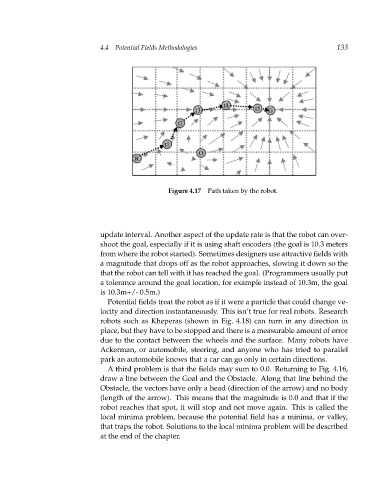
Figure 4.17 Path taken by the robot. 133

update interval. Another aspect of the update rate is that the robot can over-
shoot the goal, especially if it is using shaft encoders (the goal is 10.3 meters
from where the robot started). Sometimes designers use attractive fields with
a magnitude that drops off as the robot approaches, slowing it down so the
that the robot can tell with it has reached the goal. (Programmers usually put
a tolerance around the goal location, for example instead of 10.3m, the goal
is 10.3m+/- 0.5m.)
Potential fields treat the robot as if it were a particle that could change ve-
locity and direction instantaneously. This isn’t true for real robots. Research
robots such as Kheperas (shown in Fig. 4.18) can turn in any direction in
place, but they have to be stopped and there is a measurable amount of error
due to the contact between the wheels and the surface. Many robots have
Ackerman, or automobile, steering, and anyone who has tried to parallel
park an automobile knows that a car can go only in certain directions.
A third problem is that the fields may sum to 0.0. Returning to Fig. 4.16,
draw a line between the Goal and the Obstacle. Along that line behind the
Obstacle, the vectors have only a head (direction of the arrow) and no body
(length of the arrow). This means that the magnitude is 0.0 and that if the
robot reaches that spot, it will stop and not move again. This is called the
local minima problem, because the potential field has a minima, or valley,
that traps the robot. Solutions to the local minima problem will be described
at the end of the chapter.