Page 310 - Introduction to Autonomous Mobile Robots

Planning and Navigation

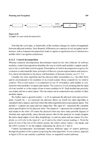
action perceptual 295
r
specification output

Figure 6.20
Example of a pure serial decomposition.

Note that the cycle time, or bandwidth, of the modules changes by orders of magnitude
between adjacent modules. Such dramatic differences are common in real navigation archi-
tectures, and so temporal decomposition tends to capture a significant axis of variation in a
mobile robot’s navigation architecture.

6.3.3.2 Control decomposition
Whereas temporal decomposition discriminates based on the time behavior of software
modules, control decomposition identifies the way in which each module’s output contrib-
utes to the overall robot control outputs. Presentation of control decomposition requires the
evaluator to understand the basic principles of discrete systems representation and analysis.
For a lucid introduction to the theory and formalism of discrete systems, see [17, 71].
Consider the robot algorithm and the physical robot instantiation (i.e., the robot form
and its environment) to be members of an overall system whose connectivity we wish to
S
examine. This overall system is comprised of a set M of modules, each module m con-
nected to other modules via inputs and outputs. The system is closed, meaning that the input
of every module m is the output of one or more modules in M . Each module has precisely
one output and one or more inputs. The one output can be connected to any number of other
modules inputs.
r
We further name a special module in M to represent the physical robot and environ-
ment. Usually by we represent the physical object on which the robot algorithm is
r
intended to have impact, and from which the robot algorithm derives perceptual inputs. The
r
r
module contains one input and one output line. The input of represents the complete
action specification for the physical robot. The output of represents the complete percep-
r
tual output to the robot. Of course the physical robot may have many possible degrees of
freedom and, equivalently, many discrete sensors. But for this analysis we simply imagine
the entire input/output vector, thus simplifying r to just one input and one output. For sim-
plicity we will refer to the input of as O and to the robot’s sensor readings . From the
I
r
I
point of view of the rest of the control system, the robot’s sensor values are inputs, and
the robot’s actions O are the outputs, explaining our choice of and O .
I
Control decomposition discriminates between different types of control pathways
through the portion of this system comprising the robot algorithm. At one extreme, depicted
in figure 6.20 we can consider a perfectly linear, or sequential control pathway.