Page 66 - Introduction to Autonomous Mobile Robots

Mobile Robot Kinematics

Y I 51
castor wheel
v(t)
θ

ω(t)
X I

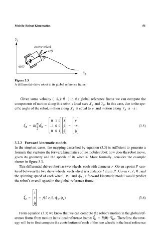
Figure 3.3
A differential-drive robot in its global reference frame.

Given some velocity ( x y θ,, · ) in the global reference frame we can compute the
· ·
components of motion along this robot’s local axes X R and Y R . In this case, due to the spe-
·
cific angle of the robot, motion along X is equal to and motion along Y is x– · :
y
R R
01 0 x · y ·
· π · · ·
ξ = R ---()ξ = –0 0 y = x – (3.5)
1
R I
2 · ·
00 1 θ θ
3.2.2 Forward kinematic models
In the simplest cases, the mapping described by equation (3.3) is sufficient to generate a
formula that captures the forward kinematics of the mobile robot: how does the robot move,
given its geometry and the speeds of its wheels? More formally, consider the example
shown in figure 3.3.
This differential drive robot has two wheels, each with diameter . Given a point cen-
P
r
r l θ
tered between the two drive wheels, each wheel is a distance from . Given , , , and
P
l
the spinning speed of each wheel, ϕ · and ϕ · , a forward kinematic model would predict
1 2
the robot’s overall speed in the global reference frame:
x ·
· ·
ξ = y = flr θϕ ϕ,, ,( · 1 , · 2 ) (3.6)
I
θ ·
From equation (3.3) we know that we can compute the robot’s motion in the global ref-
· ·
–
1
erence frame from motion in its local reference frame: ξ = R θ() ξ R . Therefore, the strat-
I
egy will be to first compute the contribution of each of the two wheels in the local reference