Page 68 - Introduction to Autonomous Mobile Robots

53
Mobile Robot Kinematics
We can now use this kinematic model in an example. However, we must first compute
R θ() – 1 . In general, calculating the inverse of a matrix may be challenging. In this case,
· ·
however, it is easy because it is simply a transform from ξ R to ξ I rather than vice versa:

cos θ – sin θ 0
– 1
R θ() = sin θ cos θ 0 (3.10)
0 0 1

⁄
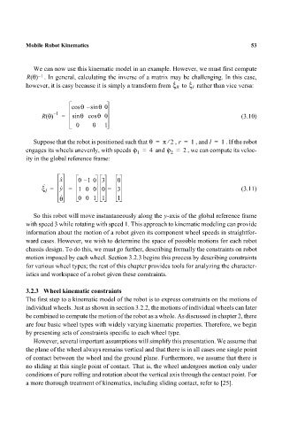
Suppose that the robot is positioned such that θ = π 2 , r = 1 , and l = 1 . If the robot
·
·
engages its wheels unevenly, with speeds ϕ = 4 and ϕ = 2 , we can compute its veloc-
1 2
ity in the global reference frame:
x · 01–0 3 0
· ·
ξ = y = 100 0 = 3 (3.11)
I
θ · 001 1 1

So this robot will move instantaneously along the y-axis of the global reference frame
with speed 3 while rotating with speed 1. This approach to kinematic modeling can provide
information about the motion of a robot given its component wheel speeds in straightfor-
ward cases. However, we wish to determine the space of possible motions for each robot
chassis design. To do this, we must go further, describing formally the constraints on robot
motion imposed by each wheel. Section 3.2.3 begins this process by describing constraints
for various wheel types; the rest of this chapter provides tools for analyzing the character-
istics and workspace of a robot given these constraints.

3.2.3 Wheel kinematic constraints
The first step to a kinematic model of the robot is to express constraints on the motions of
individual wheels. Just as shown in section 3.2.2, the motions of individual wheels can later
be combined to compute the motion of the robot as a whole. As discussed in chapter 2, there
are four basic wheel types with widely varying kinematic properties. Therefore, we begin
by presenting sets of constraints specific to each wheel type.
However, several important assumptions will simplify this presentation. We assume that
the plane of the wheel always remains vertical and that there is in all cases one single point
of contact between the wheel and the ground plane. Furthermore, we assume that there is
no sliding at this single point of contact. That is, the wheel undergoes motion only under
conditions of pure rolling and rotation about the vertical axis through the contact point. For
a more thorough treatment of kinematics, including sliding contact, refer to [25].