Page 67 - Introduction to Autonomous Mobile Robots

52
· Chapter 3
frame, ξ R . For this example of a differential-drive chassis, this problem is particularly
straightforward.
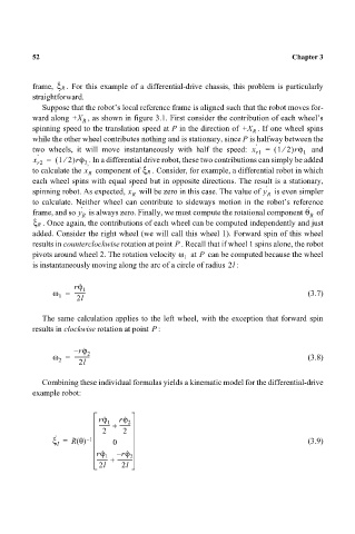
Suppose that the robot’s local reference frame is aligned such that the robot moves for-
ward along +X , as shown in figure 3.1. First consider the contribution of each wheel’s
R
spinning speed to the translation speed at P in the direction of +X R . If one wheel spins
while the other wheel contributes nothing and is stationary, since P is halfway between the
·
⁄
two wheels, it will move instantaneously with half the speed: x r1 = ( 12)rϕ · 1 and
· ·
⁄
x = ( 12)rϕ . In a differential drive robot, these two contributions can simply be added
r2 2 ·
·
to calculate the x R component of ξ R . Consider, for example, a differential robot in which
each wheel spins with equal speed but in opposite directions. The result is a stationary,
· ·
spinning robot. As expected, x will be zero in this case. The value of y is even simpler
R R
to calculate. Neither wheel can contribute to sideways motion in the robot’s reference
· ·
frame, and so y R is always zero. Finally, we must compute the rotational component θ R of
·
ξ R . Once again, the contributions of each wheel can be computed independently and just
added. Consider the right wheel (we will call this wheel 1). Forward spin of this wheel
results in counterclockwise rotation at point . Recall that if wheel 1 spins alone, the robot
P
pivots around wheel 2. The rotation velocity ω 1 at can be computed because the wheel
P
is instantaneously moving along the arc of a circle of radius 2l :
rϕ ·
ω = -------- 1 (3.7)
1 2l
The same calculation applies to the left wheel, with the exception that forward spin
P
results in clockwise rotation at point :
r – ϕ · 2
ω = ----------- (3.8)
2
2l
Combining these individual formulas yields a kinematic model for the differential-drive
example robot:

rϕ · rϕ ·
1
-------- + -------- 2
2 2
·
ξ = R θ() – 1 (3.9)
I 0
rϕ 1 r – ϕ · 2
·
-------- + -----------
2l 2l