Page 93 - Introduction to Autonomous Mobile Robots

78

Y I Chapter 3

x, y, θ

y(t)
x(t)
θ(t)
X I
1 2 3 t / [s]
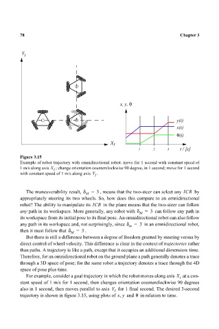
Figure 3.15
Example of robot trajectory with omnidirectional robot: move for 1 second with constant speed of
1 m/s along axis X ; change orientation counterclockwise 90 degree, in 1 second; move for 1 second
I
with constant speed of 1 m/s along axis Y .
I
The maneuverability result, δ M = 3 , means that the two-steer can select any ICR by
appropriately steering its two wheels. So, how does this compare to an omnidirectional
robot? The ability to manipulate its ICR in the plane means that the two-steer can follow
any path in its workspace. More generally, any robot with δ = 3 can follow any path in
M
its workspace from its initial pose to its final pose. An omnidirectional robot can also follow
any path in its workspace and, not surprisingly, since δ m = 3 in an omnidirectional robot,
then it must follow that δ = . 3
M
But there is still a difference between a degree of freedom granted by steering versus by
direct control of wheel velocity. This difference is clear in the context of trajectories rather
than paths. A trajectory is like a path, except that it occupies an additional dimension: time.
Therefore, for an omnidirectional robot on the ground plane a path generally denotes a trace
through a 3D space of pose; for the same robot a trajectory denotes a trace through the 4D
space of pose plus time.
For example, consider a goal trajectory in which the robot moves along axis X I at a con-
stant speed of 1 m/s for 1 second, then changes orientation counterclockwise 90 degrees
also in 1 second, then moves parallel to axis Y I for 1 final second. The desired 3-second
θ
trajectory is shown in figure 3.15, using plots of xy, and in relation to time.