Page 183 - Introduction to Computational Fluid Dynamics

P1: IWV
CB908/Date
0 521 85326 5
0521853265c06
162
2D CONVECTION – COMPLEX DOMAINS
R May 25, 2005 11:10
X 2
East
X 1 Channel
North
Wall
Central Rod
r 0
West South
b 1
b 2
Figure 6.1. Example of a complex domain.

coordinates to curvilinear coordinates via transformation relations

x 1 = F 1 (ξ 1 ,ξ 2 ), x 2 = F 2 (ξ 1 ,ξ 2 ). (6.1)
In general, these functional relationships must be developed by numerical grid
generation techniques (see Chapter 8). The grids shown in Figure 6.2 are in fact
generated by numerical means. For simpler domains, however, the functional rela-
tionships can be specified by algebraic functions. The new set of transport equations
in curvilinear coordinates are developed in Section 6.2.
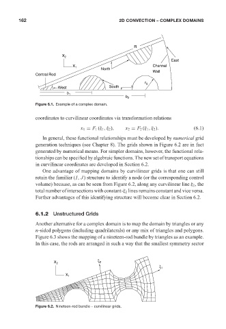
One advantage of mapping domains by curvilinear grids is that one can still
retain the familiar (I, J) structure to identify a node (or the corresponding control
volume) because, as can be seen from Figure 6.2, along any curvilinear line ξ 1 , the
total number of intersections with constant-ξ 2 lines remains constant and vice versa.
Further advantages of this identifying structure will become clear in Section 6.2.

6.1.2 Unstructured Grids

Another alternative for a complex domain is to map the domain by triangles or any
n-sided polygons (including quadrilaterals) or any mix of triangles and polygons.
Figure 6.3 shows the mapping of a nineteen-rod bundle by triangles as an example.
In this case, the rods are arranged in such a way that the smallest symmetry sector

ξ
X 2 2
ξ 1
X 1

Figure 6.2. Nineteen-rod bundle – curvilinear grids.