Page 184 - Introduction to Computational Fluid Dynamics

P1: IWV
CB908/Date
0 521 85326 5
0521853265c06
6.1 INTRODUCTION

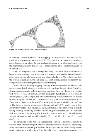
Figure 6.3. Nineteen-rod bundle – unstructured grid. May 25, 2005 11:10 163

is a doubly connected domain. Such mapping can be generated by commercially
available grid generators such as ANSYS. Each triangle may now be viewed as a
control volume over which the transport equations are to be integrated to arrive at
the discretised equations. The process of generating the latter equations is described
in Section 6.3.
It will be recognized that a triangle is a very convenient elemental construct
because it can map any convex intrusion or concave extrusion at the domain bound-
aries.Moreimportantly,trianglescanalsoeffectivelyskirtanyblockedregionwithin
the overall domain, as shown in Figure 6.3. Such skirting cannot be elegantly ac-
complished if curvilinear grids are used for mapping.
The flexibility offered by mapping by triangulation is thus obvious. Further, it is
not necessary that all triangles be of the same size or shape. In spite of this flexibility,
it becomes necessary to make a significant departure from curvilinear grid practise
with respect to node identification when unstructured grids are used. It is obvious
from Figure 6.3, for example, that one cannot readily identify elements (or nodes)
by employing the familiar (I, J) structure as was possible with curvilinear grids.
Elements, perforce, must be identified serially with a single identifier N (say). As
will be shown in Section 6.3, commercial codes such as ANSYS identify elements in
any arbitrary order. Thus, an element having identifier N will interact with elements
having arbitrary identifying numbers without any generalisable rules. This contrasts
with the case of curvilinear grids in which a control volume (I, J) will always
interact with control volumes identified by (I + 1, J), (I − 1, J), (I, J + 1), and
(I, J − 1).
This serial numbering has consequences for solution of discretised equations
evolved on an unstructured grid. This will become clearer in Section 6.3. In passing,
we note that there are a variety of methods for triangulation. Automatic triangulation
requires detailed considerations from the subject of computational geometry. In