Page 189 - Introduction to Computational Fluid Dynamics

P1: IWV
0 521 85326 5
11:10
May 25, 2005
0521853265c06
CB908/Date
168
ξ 2 2D CONVECTION – COMPLEX DOMAINS
NE
N
ne
NW
n
nw
E
e
P
U f1
X 2
se
ξ 1
w
W
s U f2
SE
sw
X 1
S
SW
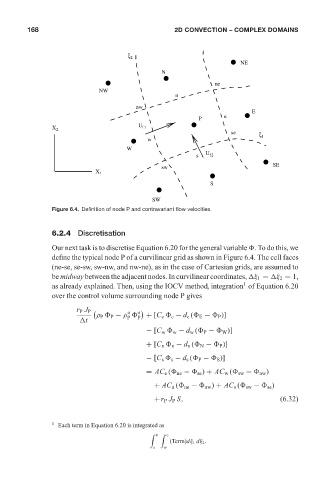
Figure 6.4. Definition of node P and contravariant flow velocities.

6.2.4 Discretisation

Our next task is to discretise Equation 6.20 for the general variable . To do this, we
define the typical node P of a curvilinear grid as shown in Figure 6.4. The cell faces
(ne-se, se-sw, sw-nw, and nw-ne), as in the case of Cartesian grids, are assumed to
be midway between the adjacent nodes. In curvilinear coordinates, ξ 1 = ξ 2 = 1,
1
as already explained. Then, using the IOCV method, integration of Equation 6.20
over the control volume surrounding node P gives
r P J P
o o
ρ P P − ρ + [C e e − d e ( E − P )]
t P P
− [C w w − d w ( P − W )]
+ [C n n − d n ( N − P )]

− [C s s − d s ( P − S )]
= AC e ( ne − se ) + AC w ( sw − nw )

+ AC n ( ne − nw ) + AC s ( sw − se )
+r P J P S, (6.32)

1
Each term in Equation 6.20 is integrated as
n e

(Term)dξ 1 dξ 2 .
s w