Page 193 - Introduction to Computational Fluid Dynamics

P1: IWV
CB908/Date
May 25, 2005
0521853265c06
11:10
172
J = JN 0 521 85326 5 2D CONVECTION – COMPLEX DOMAINS
o o o o o o o o
o NORTH
o o
WEST 5 o o o o
o
o
o o o o o o o o
J = 1 o o
I = 1 2 3 8 o o
12 o
o
o
o
IN = 31
16 o o
JN = 9 SOUTH
o
o o
20 o
I = IN 30 24 o o
J = 1 o
o o o o o o o o o
o
o
EAST 5 o o o
o o o o
o o o o o o o o
J = JN
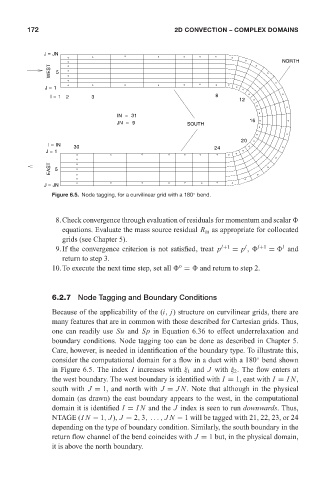
Figure 6.5. Node tagging, for a curvilinear grid with a 180 bend.
◦
8.Check convergence through evaluation of residuals for momentum and scalar
equations. Evaluate the mass source residual R m as appropriate for collocated
grids (see Chapter 5).
l
l
9.If the convergence criterion is not satisfied, treat p l+1 = p , l+1 = and
return to step 3.
o
10.To execute the next time step, set all = and return to step 2.
6.2.7 Node Tagging and Boundary Conditions
Because of the applicability of the (i, j) structure on curvilinear grids, there are
many features that are in common with those described for Cartesian grids. Thus,
one can readily use Su and Sp in Equation 6.36 to effect underrelaxation and
boundary conditions. Node tagging too can be done as described in Chapter 5.
Care, however, is needed in identification of the boundary type. To illustrate this,
consider the computational domain for a flow in a duct with a 180 bend shown
◦
in Figure 6.5. The index I increases with ξ 1 and J with ξ 2 . The flow enters at
the west boundary. The west boundary is identified with I = 1, east with I = IN,
south with J = 1, and north with J = JN. Note that although in the physical
domain (as drawn) the east boundary appears to the west, in the computational
domain it is identified I = IN and the J index is seen to run downwards. Thus,
NTAGE (IN − 1, J), J = 2, 3, ..., JN − 1 will be tagged with 21, 22, 23, or 24
depending on the type of boundary condition. Similarly, the south boundary in the
return flow channel of the bend coincides with J = 1 but, in the physical domain,
it is above the north boundary.