Page 194 - Introduction to Computational Fluid Dynamics

P1: IWV
0 521 85326 5
CB908/Date
0521853265c06
6.2 CURVILINEAR GRIDS
ξ 2 May 25, 2005 11:10 173
nw
n
∆n
(1, J)
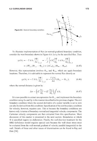
Figure 6.6. Gradient boundary condition. (2, J)
e
Flux q
1, J
sw ξ 1
s

To illustrate implementation of flux (or normal-gradient) boundary condition,
consider the west boundary shown in Figure 6.6. Let q be the specified flux. Then

∂ ∂
∂ 2
qd A 1 =−
dA 1 =− dA 1 + dA 12
∂n J
(1, j) ∂ξ 1 ∂ξ 2 (1, j)
= AW 2, j ( 1, j − 2, j ) + (AC w ) 2, j ( sw − nw ). (6.45)
However, this representation involves sw and nw , which are again boundary
locations. Therefore, it is advisable to represent the normal flux directly as

∂
dA 1
qd A 1 =−
dA 1 =− ( 2, j − 1, j ), (6.46)
∂n n
(1, j)
where the normal distance is given by
'
n = β i 1 ∂x 1 + β i 2 ∂x 2 dA i . (6.47)
∂ξ i ∂ξ i
It is now possible to extract an expression for 1, j and implement the boundary
condition using Su and Sp in the manner described in the previous chapter. The exit
boundary condition where the second derivative of a scalar variable is set to zero
can also be derived from this condition. Specification of the exit boundary condition
for velocity, however, requires care. This is because the boundary conditions are
known only in terms of boundary-normal and tangential velocity components. The
Cartesian velocity components are then extracted from this specification. More
discussion of this matter is presented in the next section. Boundaries at which
is specified require no elaboration. Finally, the wall-function treatment for the
HRE turbulence model requires special care because the wall shear stress must
be evaluated from the wall-normal gradient of velocity parallel (tangential) to the
wall. Details of these and other issues of discretisation can be found in Ray and
Date [58].