Page 199 - Introduction to Computational Fluid Dynamics

P1: IWV
CB908/Date
0 521 85326 5
0521853265c06
178
2D CONVECTION – COMPLEX DOMAINS
ξ 2 May 25, 2005 11:10
b n
ξ 2 n
b
c
c
a ξ 1
P e ξ 1 e E
E P
a
(a) (b)
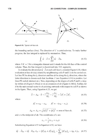
Figure 6.10. Typical cell face ab.

the bounding surface (line). The direction of C is anticlockwise. To make further
progress, the line integral is replaced by summation. Thus,

NK

q

q · A = ( · A) k , (6.52)
C k=1
where NK = 3 for a triangular element and k stands for the kth face of the control
volume. Thus, the line integral is discretized into NK segments.
To evaluate the dot product · A at each cell face k, consider Figure 6.10, where
q

evaluation at face ab (say) shared by neighbouring cells P and E is to be carried out.
Let line PE be along the ξ 1 direction and line ab be along the ξ 2 direction, where the
latter direction is chosen such that Jacobian J (see Equation 6.14) is positive. Let
lines PE and ab intersect at e. Now, depending on the shapes of cells P and E, e may
lie within ab [Figure 6.10(a)] or on an extension of ab [Figure 6.10(b)]. Further, let
n be the unit normal vector to ab pointing outwards with respect to cell P as shown
in the figure. Then, using Equation 6.25, we get
∂x 2 ∂x 1 1 2
A = A ab · n = i − j = i β + j β , (6.53)

1
1
∂ξ 2 ∂ξ 2
where
1
2
β = x 2b − x 2a , β =−(x 1b − x 1a ), (6.54)
1 1
%

1 2
2 2
A ab = A ck = β + β = area of face ab, (6.55)
1 1
and c is the midpoint of ab. The coordinates of c are
1
x i,c = (x i,a + x i,b ). (6.56)
2
Substituting Equation 6.53 in Equation 6.52, we have
2

1 2
i
q = = (q n A c ) k . (6.57)
( · A) ck = ( q · n) ck A ck = β q 1 + β q 2 β q i
1 1 k 1 k
i=1