Page 202 - Introduction to Computational Fluid Dynamics

P1: IWV
CB908/Date
0 521 85326 5
0521853265c06
6.3 UNSTRUCTURED MESHES
where, following Equation 6.60, May 25, 2005 11:10 181
1 2

C ck = ρ ck β u 1 + β u 2 ck . (6.65)
1
1
Now, ρ ck , u 1,ck , and u 2,ck are linearly interpolated according to the following general
formula: 4
]. (6.66)
ck = [ f m,c E 2 + (1 − f m,c ) P 2
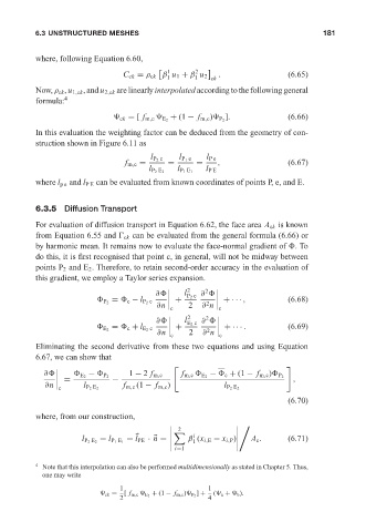
In this evaluation the weighting factor can be deduced from the geometry of con-
struction shown in Figure 6.11 as
l P 2 c l P 1 e l Pe
f m,c = = = , (6.67)
l PE
l P 2 E 2 l P 1 E 1
where l pe and l PE can be evaluated from known coordinates of points P, e, and E.

6.3.5 Diffusion Transport

For evaluation of diffusion transport in Equation 6.62, the face area A ck is known
from Equation 6.55 and
ck can be evaluated from the general formula (6.66) or
by harmonic mean. It remains now to evaluate the face-normal gradient of .To
do this, it is first recognised that point c, in general, will not be midway between
points P 2 and E 2 . Therefore, to retain second-order accuracy in the evaluation of
this gradient, we employ a Taylor series expansion.

l
2 2
∂ P 2 c ∂
= c − l P 2 c + +· · · , (6.68)
P 2
∂n 2 ∂ n
2
c c
l
2 2
∂ E 2 c ∂
= c + l E 2 c + +· · · . (6.69)
E 2
∂n 2 ∂ n
2
c c
Eliminating the second derivative from these two equations and using Equation
6.67, we can show that

∂ E 2 − P 2 1 − 2 f m,c f m,c E 2 − c + (1 − f m,c ) P 2
= − ,
∂n f m,c (1 − f m,c )
c l P 2 E 2 l P 2 E 2
(6.70)
where, from our construction,
(
2
i
n (6.71)
1
l P 2 E 2 = l P 1 E 1 A c .
β (x i,E − x i,P )
= l PE · =
i=1

4 Note that this interpolation can also be performed multidimensionally as stated in Chapter 5. Thus,
one may write
1 1
ck = [ f m,c E 2 + (1 − f m,c ) P 2 ] + ( a + b ).
2 4