Page 203 - Introduction to Computational Fluid Dynamics

P1: IWV
0 521 85326 5
May 25, 2005
11:10
CB908/Date
0521853265c06
182
2D CONVECTION – COMPLEX DOMAINS
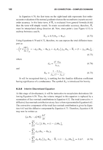
In Equation 6.70, the first term on the right-hand side represents first-order-
accurate evaluation of the normal gradient whereas the second term imparts second-
order accuracy. In this latter term, if c is evaluated from general formula (6.66)
then the term will simply vanish. To retain second-order accuracy, therefore, c
must be interpolated along direction ab. Now, since point c (see Figure 6.11) is
midway between a and b,
ck = 0.5( ak + bk ). (6.72)
Using Equations 6.70 and 6.72, therefore, we can express the total diffusion trans-
port as

∂
)
−
A =−d ck ( E 2 − P 2 k + d ck B ck f m,c E 2 − c + (1 − f m,c ) P 2 k ,
∂n ck
(6.73)
where
(
A) ck
d ck = (6.74)
l P 2 E 2
and
1 − 2 f m,c
B ck = . (6.75)
f m,c (1 − f m,c )
It will be recognised that d ck is nothing but the familiar diffusion coefficient
having significance of a conductance. The symbol B ck is introduced for brevity.

6.3.6 Interim Discretised Equation
At this stage of development, it will be instructive to recapitulate derivations fol-
lowing Equation 6.50. Thus, the volume integral in this equation is replaced by a
summation of face-normal contributions in Equation 6.52. The total (convective +
diffusive) face-normal contribution at any face is then represented in Equation 6.62.
The convective component of the total face-normal contribution is given by Equa-
tion 6.63 and the diffusive component by Equation 6.73. Therefore, Equation 6.50
may now be written as
V

o o
ρ P P − ρ P
P
t
NK

+ C ck f c P 2 + (1 − f c ) E 2 k
k=1
NK

)
− d ck ( E 2 − P 2 k
k=1
NK

+ d ck B ck f m,c E 2 − c + (1 − f m,c ) P 2 k = S V. (6.76)
k=1