Page 208 - Introduction to Computational Fluid Dynamics

P1: IWV
0 521 85326 5
CB908/Date
0521853265c06
6.3 UNSTRUCTURED MESHES
b INFLUX F B May 25, 2005 11:10 187
n
ξ
ξ 2 1
B = c = e
BOUNDARY FACE
P
P 2
a

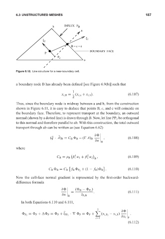
Figure 6.12. Line structure for a near-boundary cell.

a boundary node B has already been defined [see Figure 6.9(b)] such that

1
x i,B = (x i,a + x i,b ). (6.107)
2

Thus, since the boundary node is midway between a and b, from the construction
shown in Figure 6.11, it is easy to deduce that points B, c, and e will coincide on
the boundary face. Therefore, to represent transport at the boundary, an outward
normal (shown by a dotted line) is drawn through B. Now, let line PP 2 be orthogonal
to this normal and therefore parallel to ab. With this construction, the total outward
transport through ab can be written as (see Equation 6.62)

∂
q , (6.108)
( · A) B = C B B − (
A) B
∂n
B
where
1 2

C B = ρ B β u 1 + β u 2 B , (6.109)
1
1

+ (1 − f B ) B . (6.110)
C B B = C B f B P 2
Now the cell-face normal gradient is represented by the first-order backward-
difference formula

)
∂ ( B − P 2
= . (6.111)
∂n B l P 2 B
In both Equations 6.110 and 6.111,
2

∂
− x i,P ) .
P 2 = P + P = P + l PP 2 ·∇ P = P + (x i,P 2

i=1 ∂x i P
(6.112)