Page 212 - Introduction to Computational Fluid Dynamics

P1: IWV
CB908/Date
0 521 85326 5
0521853265c06
6.3 UNSTRUCTURED MESHES
c 3 May 25, 2005 11:10 191
n
b
E 2
c 4
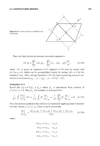
Figure 6.13. Construction of a cell-face con- c
trol volume.
c 2

P 2
a

c 1

Thus, the final discretised pressure correction equation is

NK NK
V

o
AP p = AE k p − C ck − ρ P − ρ , (6.134)
P Ek P
k=1 k=1 t
where AE k is given by Equation 6.133. Equation 6.134 must be solved with
∂p /∂n | B = 0, which can be accomplished simply by setting AE k = 0 for the

boundary face. After solving Equation 6.134, the mass-conserving pressure cor-
l
l

rection is recovered as p = p − p = p − 0.5(p − p ).
m sm
Evaluation of p
Recall that p = 0.5(p + p ), where p is determined from solution of
P x 1 x 2 x i
2
2
∂ p/∂x | P = 0. Thus p , for example, is evaluated from
i x 1
NK
2
1 ∂ p 1 1 ∂p 1 1 ∂p
dV = β = β = 0. (6.135)
1 1
V ∂x 2 V C ∂x 1 ck V ∂x 1 ck

1 P k=1
Now, the pressure gradient at the cell face is evaluated by applying Gauss’s theorem
over the volume c 1 –c 2 –c 3 –c 4 . Then, it can be shown that

∂p x 2,E 2 p E 2 + x 2,b p b + x 2,P 2 p P 2 + x 2,a p a
= , (6.136)

∂x 1 ck V ck
where
),
x 2,E 2 = (x 2,c 3 − x 2,c 2
),
x 2,b = (x 2,c 4 − x 2,c 3
),
x 2,P 2 = (x 2,c 1 − x 2,c 4
).
x 2,a = (x 2,c 2 − x 2,c 1