Page 210 - Introduction to Computational Fluid Dynamics

P1: IWV
0 521 85326 5
May 25, 2005
0521853265c06
CB908/Date
6.3 UNSTRUCTURED MESHES
These two types of scalar boundary conditions typically suffice to affect physical 11:10 189
conditions at inflow, wall, exit, and symmetry boundaries of the domain.
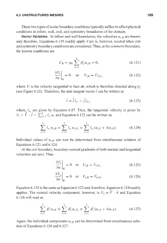
Vector Variables: At inflow and wall boundaries, the velocities u i,B are known
and, therefore, Equations 6.119 readily apply. Care is, however, needed when exit
and symmetry boundary conditions are considered. Thus, at thesymmetry boundary,
the known conditions are
2
i
C B = ρ B β u i,B = 0, (6.121)
1
i=1

∂V t
= 0 or , (6.122)
V t,B = V t,P 2
∂n B
where V t is the velocity tangential to face ab, which is therefore directed along ξ 2
(see Figure 6.12). Therefore, the unit tangent vector t can be written as

t = il x 1 + jl x 2 , (6.123)
are given by Equation 6.87. Thus, the tangential velocity is given by
where, l x i
2

V t = V · t = l u i and Equation 6.122 can be written as
i=1 x i
2 2 2

u i,B = = (u i,P + u i,P ). (6.124)
l x i l x i u i,P 2 l x i
i=1 i=1 i=1
Individual values of u i,B can now be determined from simultaneous solution of
Equations 6.121 and 6.124.
At the exit boundary, boundary-normal gradients of both normal and tangential
velocities are zero. Thus

∂V t
= 0or (6.125)
V t,B = V t,P 2 ,
∂n B

∂V n
= 0or . (6.126)
V n,B = V n,P 2
∂n
B
Equation 6.125 is the same as Equation 6.122 and, therefore, Equation 6.124 readily
applies. The normal velocity component, however, is V n = V · n and Equation

6.126 will read as
2 2 2

i i i
β u i,B = = β (u i,P + u i,P ). (6.127)
1 β u i,P 2 1
1
i=1 i=1 i=1
Again, the individual components u i,B can be determined from simultaneous solu-
tion of Equations 6.124 and 6.127.