Page 213 - Introduction to Computational Fluid Dynamics

P1: IWV
0 521 85326 5
May 25, 2005
11:10
0521853265c06
CB908/Date
192
However, note that 2D CONVECTION – COMPLEX DOMAINS
= x 2,b − x 2,a = β 1
1
x 2,E 2 =− x 2,P 2
and
(
2

i 2
2 A .
1 β (x i,E − x i,P ) c
1
x 2,a =− x 2,b = x 2,E 2 − x 2,P 2 = x 2,E 1 − x 2,P 1
= β
i=1

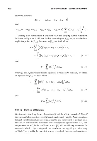
Making these substitutions in Equation 6.136 and carrying out the summation
indicated in Equation 6.135, and further separating out p x1,P = p P , we obtain an
explicit equation for p x1,P that reads as p x 1 ,P = A/B, where
NK )
A =
β 1 2 (p E + p E − p P ) *# V ck
1
k=1
NK
1 &

− )(p b − p a ) V ck , (6.137)
1 − x 2,P 2
β (x 2,E 2
k=1
and
NK 2 #

B = β 1 1 V ck , (6.138)
k=1
where p b and p a are evaluated using Equations 6.92 and 6.93. Similarly, we obtain
an equation for p x 2 ,P = A/B, where
NK )
2 2 *#

A = β (p E + p E − p P ) V ck
1
k=1
NK
2 &

− )(p b − p a ) (6.139)
1 − x 1,P 2 V ck
β (x 1,E 2
k=1
and
NK 2 #

B = β 2 1 V ck . (6.140)
k=1
6.3.12 Method of Solution
Our interest is in solving the set of equations (6.103) for all interior nodes P. Thus, if
there are NE elements, there are NE equations for each variable. Again, equations
for each variable are solved sequentially (see the next subsection). It has been noted
that the AP coefficients will dominate over the neighbouring coefficients AE k . But,
the positions of AE k in the coefficient matrix [A] will be arbitrary because of the
manner in which neighbouring nodes are numbered during grid generation using
ANSYS. This is unlike the case of structured grids (both Cartesian and curvilinear)