Page 217 - Introduction to Computational Fluid Dynamics

P1: IWV
11:10
May 25, 2005
CB908/Date
0521853265c06
196
1000 0 521 85326 5 2D CONVECTION – COMPLEX DOMAINS
Grimison

Zhukauskas
100

f x 10 3 Nu

10

INLINE ARRAY

1
10 100 1000 10000 100000 1E6
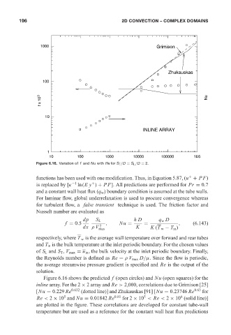
Figure 6.16. Variation of f and Nu with Re for S T /D = S L /D = 2.

+
functions has been used with one modification. Thus, in Equation 5.87, (u + PF)
+
is replaced by [κ −1 ln(Ey ) + PF]. All predictions are performed for Pr = 0.7
and a constant wall heat flux (q w ) boundary condition is assumed at the tube walls.
For laminar flow, global underrelaxation is used to procure convergence whereas
for turbulent flow, a false transient technique is used. The friction factor and
Nusselt number are evaluated as
dp S L hD q w D
f = 0.5 , Nu = = , (6.143)
2
dx ρ V max K K (T w − T in )
respectively, where T w is the average wall temperature over forward and rear tubes
and T in is the bulk temperature at the inlet periodic boundary. For the chosen values
of S L and S T , V max = u in , the bulk velocity at the inlet periodic boundary. Finally,
the Reynolds number is defined as Re = ρ V max D/µ. Since the flow is periodic,
the average streamwise pressure gradient is specified and Re is the output of the
solution.
Figure 6.16 shows the predicted f (open circles) and Nu (open squares) for the
inline array. For the 2 × 2 array and Re > 2,000, correlations due to Grimison [25]
[Nu = 0.229 Re 0.632 (dotted line)] and Zhukauskas [91] [Nu = 0.23746 Re 0.63 for
6
5
5
Re < 2 × 10 and Nu = 0.01842 Re 0.81 for 2 × 10 < Re < 2 × 10 (solid line)]
are plotted in the figure. These correlations are developed for constant tube-wall
temperature but are used as a reference for the constant wall heat flux predictions