Page 255 - Introduction to Computational Fluid Dynamics

P1: KsF/ICD
May 10, 2005
CB908/Date
16:28
0 521 85326 5
0521853265c08
234
(a) NUMERICAL GRID GENERATION
(b)
1.0 1.0
N = 11
N = 11
0.8 0.8
n = 2.0
n = 0.5
0.6 0.6

X(I)/L X(I)/L n = 1
0.4 n = 1 n = 2.0 0.4 n = 0.5
0.2 0.2
GRID NUMBER GRID NUMBER
0.0 0.0
2 4 6 8 10 2 4 6 8 10
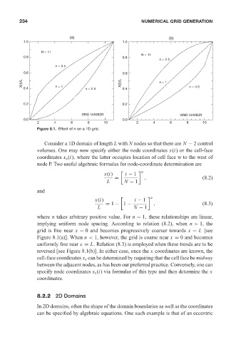
Figure 8.1. Effect of n ona1D grid.

Consider a 1D domain of length L with N nodes so that there are N − 2 control
volumes. One may now specify either the node coordinates x(i) or the cell-face
coordinates x c (i), where the latter occupies location of cell face w to the west of
node P. Two useful algebraic formulas for node-coordinate determination are
x(i) i − 1 n
= , (8.2)
L N − 1
and
n
x(i) i − 1

= 1 − 1 − , (8.3)
L N − 1
where n takes arbitrary positive value. For n = 1, these relationships are linear,
implying uniform node spacing. According to relation (8.2), when n > 1, the
grid is fine near x = 0 and becomes progressively coarser towards x = L [see
Figure 8.1(a)]. When n < 1, however, the grid is coarse near x = 0 and becomes
uniformly fine near x = L. Relation (8.3) is employed when these trends are to be
reversed [see Figure 8.1(b)]. In either case, once the x coordinates are known, the
cell-face coordinates x c can be determined by requiring that the cell face be midway
between the adjacent nodes, as has been our preferred practice. Conversely, one can
specify node coordinates x c (i) via formulas of this type and then determine the x
coordinates.

8.2.2 2D Domains

In 2D domains, often the shape of the domain boundaries as well as the coordinates
can be specified by algebraic equations. One such example is that of an eccentric