Page 258 - Introduction to Computational Fluid Dynamics

P1: KsF/ICD
CB908/Date
0 521 85326 5
May 10, 2005
0521853265c08
8.3 DIFFERENTIAL GRID GENERATION
T 1 = 1 q = 0 16:28 237
n
0.9
0.7 0.8
0.6
0.3 0.5
0.6 ,1 0.9
0.4
q = 0
n 0.2 T 2 = 0
q = 0 T = 1
n 2
0.1
T 1 = 0 q = 0
n
(a) (b)

(c)
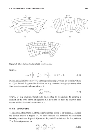
Figure 8.4. Differential construction of a 2D curvilinear grid.

taken as
b

2
x = T 1 − (1 − T ) , 0 ≤ T ≤ 1. (8.8)
6k
By assigning different values to T in the specified range, we can get as many values
of x(i) as desired. To generalise this idea, we may state that the appropriate equation
for determination of node coordinates is
2
d ξ
= c (ξ), (8.9)
dx 2
where c (ξ)isa stretching function to be specified by the analyst. To generate a
solution of the form shown in Equation 8.8, Equation 8.9 must be inverted. This
matter will be discussed in Section 8.3.3.

8.3.2 2D Domains

To understand the extension of the aforementioned notion to 2D domains, consider
the domain shown in Figure 8.4. We now consider two problems with different
boundary conditions. Figure 8.4(a) shows the probable solution to the first problem
T = T 1 (say) governed by
2 2
∂ T 1 ∂ T 1 q 1
+ = , (8.10)
∂x 2 ∂x 2 k
1 2