Page 262 - Introduction to Computational Fluid Dynamics

P1: KsF/ICD
CB908/Date
0 521 85326 5
0521853265c08
8.4 SORENSON’S METHOD
ζ
ζ 2 May 10, 2005 16:28 241
2max
∆S max
X 2

X 1

θ ∆S o
i − 1 i i + 1
ζ 2 = 0
ζ 1
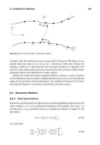
Figure 8.5. Grid line construction – Sorenson’s method.

boundary, than the problem becomes overspecified or ill-posed. Therefore, we can
specify either the value of ∂x 1 /∂ξ 2 or of x 1 . However, if only one of these two
boundary conditions is specified then the converged solutions to Equations 8.26
and 8.27 often demonstrate grid-node clustering in some portions of the domain
and highly sparse node distributions in other regions.
Ideally, one would like to have complete freedom to choose x 1 and x 2 locations
on the boundaries and yet achieve orthogonal intersection (or at any other desired
angle) of the grid lines with the boundaries. The method of Sorenson [71] allows
precisely this freedom. The method is described in the next section.

8.4 Sorenson’s Method

8.4.1 Main Specifications

Sorenson’s method permits coordinate and coordinate-gradient specification for the
same variable x 1 or x 2 at two of the four boundaries of the domain. Thus, let ξ 2 = 0
(south) and ξ 2 = ξ 2max (north) be these two boundaries as shown in Figure 8.5. We
now define

2 2 0.5
s 0 = x + x (8.29)
1 2 ξ 2 =0
or, in the limit,

0.5

2 2

ds 0 ∂x 1 ∂x 2
= + . (8.30)
d ξ 2 ∂ξ 2 ∂ξ 2
ξ 2 =0