Page 267 - Introduction to Computational Fluid Dynamics

P1: KsF/ICD
CB908/Date
May 10, 2005
0521853265c08
16:28
246
1.0 0 521 85326 5 NUMERICAL GRID GENERATION
a = b = c = d = 1.0
−6.0 −4.0 −2.0 0.0 2.0 4.0

a = b = c = d = 0.75

a = b = c = d = 0.5
X 0 X 0

a
b

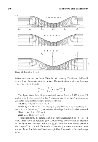
Figure 8.6. Example of H – grid.

inflow boundary, and east (x 1 = 20) is the exit boundary. The channel half-width
is b = 1 and the constriction height is δ. The constriction profile for the range
−x 0 < x 1 < x 0 is given by

δ
x 2 π x 1
= 1 − 1 + cos .
b 2b x 0
The figure shows the grid generated with s 0 = s max = 0.035, δ/b = 2/3,
and x 0 /b = 4. The grids, 32 in the ξ 1 direction and 15 in the ξ 2 direction, are
generated using the following boundary conditions.
South: x 2 = 0, for −8 < x 1 < 20.
North: x 2 = 1 for −8 < x 1 < −x 0 , x 2 = f (x 1 ) for −x 0 < x 1 < x 0 and, x 2 = 1
for x 0 < x 1 < 20, where f (x 1 ) is the constriction shape function already mentioned.
West: x 1 =−8, ∂x 2 /∂ξ 1 = 0.
East: x 1 = 20, ∂x 2 /∂ξ 1 = 0.
To maintain clarity, the generated grids are shown in Figure 8.6 for −6 < x 1 < 5
only. Three values of constants (1.0, 0.75, and 0.5) are used and are indicated
in the figure. For the largest value, the ξ 2 grid lines are more evenly spaced in
the range 0.25 < x 2 < 0.8. For smaller values, the grid nodes are attracted more
towards the north and the south boundaries, yielding fewer nodes in the middle range
of x 2 .