Page 269 - Introduction to Computational Fluid Dynamics

P1: KsF/ICD
16:28
May 10, 2005
0521853265c08
248
0.30 CB908/Date 0 521 85326 5 NUMERICAL GRID GENERATION
0.20 TRAILING EGDE
0.10

0.00

−0.10

−0.20
LEADING EDGE
PERIODIC
−0.30
BOUNDARY
−0.40
−0.25 0.00 0.25
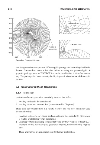
Figure 8.8. Example of O – grid.

stretching functions can produce different grid spacings and stretchings inside the
domain. One needs to make a few trials before accepting the generated grid. A
graphics package such as TECPLOT for mesh visualisation is therefore neces-
sary. The package also has a zooming facility to permit visualisation of dense-grid
regions.

8.5 Unstructured Mesh Generation

8.5.1 Main Task
Unstructured mesh generation essentially involves two tasks:

1. locating vertices in the domain and
2. creating vertex and element files (as mentioned in Chapter 6).
These tasks can be carried out in a variety of ways. The two most commonly used
are the following:

1. Locating vertices by curvilinear grid generation so that a regular (i, j) structure
is readily available for vertex numbering.
2. Locating vertices according to rules that yield arbitrary vertices without (i, j)
structure. In this automatic grid generation method, node numbering requires
care.

These alternatives are considered next for further explanation.