Page 270 - Introduction to Computational Fluid Dynamics

P1: KsF/ICD
0 521 85326 5
CB908/Date
0521853265c08
8.5 UNSTRUCTURED MESH GENERATION
I = IN = 9 May 10, 2005 16:28 249
J = JN = 5 EAST
36 27 18 9
45
44 35
26 17
43
42 8
NORTH 41
34
40
38 39
37 33
25
7
16
32
28 29
30 31 24
WEST 15
19
20 23 6
21 22
10 14
11 SOUTH
12 13
5
I = 1
J = 1
2 4
3
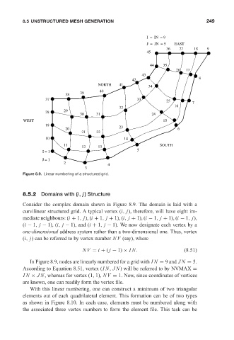
Figure 8.9. Linear numbering of a structured grid.

8.5.2 Domains with (i, j) Structure
Consider the complex domain shown in Figure 8.9. The domain is laid with a
curvilinear structured grid. A typical vertex (i, j), therefore, will have eight im-
mediate neighbours: (i + 1, j), (i + 1, j + 1), (i, j + 1), (i − 1, j + 1), (i − 1, j),
(i − 1, j − 1), (i, j − 1), and (i + 1, j − 1). We now designate each vertex by a
one-dimensional address system rather than a two-dimensional one. Thus, vertex
(i, j) can be referred to by vertex number NV (say), where

NV = i + ( j − 1) × IN. (8.51)

In Figure 8.9, nodes are linearly numbered for a grid with IN = 9 and JN = 5.
According to Equation 8.51, vertex (IN, JN) will be referred to by NVMAX =
IN × JN, whereas for vertex (1, 1), NV = 1. Now, since coordinates of vertices
are known, one can readily form the vertex file.
With this linear numbering, one can construct a minimum of two triangular
elements out of each quadrilateral element. This formation can be of two types
as shown in Figure 8.10. In each case, elements must be numbered along with
the associated three vertex numbers to form the element file. This task can be