Page 275 - Introduction to Computational Fluid Dynamics

P1: KsF/ICD
May 10, 2005
0 521 85326 5
16:28
0521853265c08
CB908/Date
254
L 1 NUMERICAL GRID GENERATION
L 2
S
t
a b
P
c d

h
g

e
f

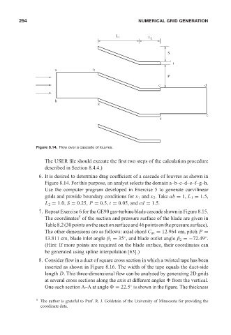
Figure 8.14. Flow over a cascade of louvres.

The USER file should execute the first two steps of the calculation procedure
described in Section 8.4.4.)
6. It is desired to determine drag coefficient of a cascade of louvres as shown in
Figure 8.14. For this purpose, an analyst selects the domain a–b–c–d–e–f–g–h.
Use the computer program developed in Exercise 5 to generate curvilinear
grids and provide boundary conditions for x 1 and x 2 . Take ab = 1, L 1 = 1.5,
L 2 = 1.0, S = 0.25, P = 0.5, t = 0.05, and cd = 1.5.
7. Repeat Exercise 6 for the GE90 gas-turbine blade cascade shown in Figure 8.15.
5
The coordinates of the suction and pressure surface of the blade are given in
Table8.2(30pointsonthesuctionsurfaceand46pointsonthepressuresurface).
The other dimensions are as follows: axial chord C ax = 12.964 cm, pitch P =
◦
13.811 cm, blade inlet angle β 1 = 35 , and blade outlet angle β 2 =−72.49 .
◦
(Hint: If more points are required on the blade surface, their coordinates can
be generated using spline interpolation [63].)
8. Consider flow in a duct of square cross section in which a twisted tape has been
inserted as shown in Figure 8.16. The width of the tape equals the duct-side
length D. This three-dimensional flow can be analysed by generating 2D grids
at several cross sections along the axis at different angles from the vertical.
◦
One such section A–A at angle = 22.5 is shown in the figure. The thickness

5 The author is grateful to Prof. R. J. Goldstein of the University of Minnesota for providing the
coordinate data.