Page 276 - Introduction to Computational Fluid Dynamics

P1: KsF/ICD
CB908/Date
0521853265c08
EXERCISES
a 0 521 85326 5 May 10, 2005 16:28 255
b
PRESSURE
SURFACE

c
h g
SUCTION
SURFACE
P

f d
Cax

e
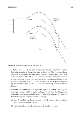
Figure 8.15. Schematic of a gas-turbine blade cascade.

of the tape δ/D = 0.04. The flow is symmetric about the tape with secondary
flow being transferred through the gaps c–d and e–f. Therefore, curvilinear
grids may be generated over only half of the duct cross section. Select west,
north, east, and south boundaries and adapt the computer program of Exercise 5
to generate the curvilinear grid. Also specify the boundary conditions for the
velocity components u i , i = 1, 2, and 3. (Hint: For the purpose of generat-
ing the curvilinear grid, assume δ = 0 to avoid any sharp protrusion into the
domain.)

9. The vertex file for the domain of Figure 8.9 is given in Table 8.3. Reading this
file, prepare an element file using the routine given in Section 8.5.2 to generate
a triangular mesh as shown in Figure 8.11. Now, with reference to Chapter 6,
develop a computer program to do the following:

(a) Identify neighboring element numbers of each element. Store this infor-
mation in array NHERE (N, K).
(b) Define boundary nodes B and assign node numbers to them.