Page 273 - Introduction to Computational Fluid Dynamics

P1: KsF/ICD
16:28
May 10, 2005
0 521 85326 5
0521853265c08
CB908/Date
252

B NUMERICAL GRID GENERATION
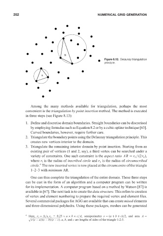
Figure 8.12. Delaunay triangulation
principle.

A

Among the many methods available for triangulation, perhaps the most
convenient is the triangulation by point insertion method. The method is executed
in three steps (see Figure 8.13):
1. Define and discretise domain boundaries. Straight boundaries can be discretised
by employing formulas such as Equation 8.2 or by a cubic-spline technique [63].
Curved boundaries, however, require further care.
2. Triangulate the boundary points using the Delaunay triangulation principle. This
creates new vertices interior to the domain.
3. Triangulate the remaining interior domain by point insertion. Starting from an
existing pair of vertices (1 and 2, say), a third vertex can be searched under a
variety of constraints. One such constraint is the aspect ratio AR = r i /(2r c ),
where r i is the radius of inscribed circle and r c is the radius of circumscribed
4
circle. The new inserted vertex is now placed at the circumcentre of the triangle
1–2–3 with minimum AR.
One can thus complete the triangulation of the entire domain. These three steps
can be cast in the form of an algorithm and a computer program can be written
for its implementation. A computer program based on a method by Watson [87] is
available in [67]. The next task is to create the data structure. This refers to creation
of vertex and element numbering to prepare the required vertex and element files.
Several commercial packages for AGG are available that can create mixed elements
and three-dimensional polyhedra. Using these packages, meshes can be generated

4
Here, r i = A/s,r c =0.25 × a × b × c/A, semiperimeter s = (a + b + c)/2, and area A =
$
s (s − a)(s − b)(s − c). a, b, and c are lengths of sides of the triangle 1-2-3.