Page 277 - Introduction to Computational Fluid Dynamics

P1: KsF/ICD
0 521 85326 5
May 10, 2005
CB908/Date
0521853265c08
256
NUMERICAL GRID GENERATION
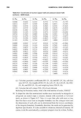
Table 8.2: Coordinates of suction (upper half) and pressure (lower half) 16:28
surfaces – GE90 blade.
x 1 /C ax x 2 /C ax x 1 /C ax x 2 /C ax x 1 /C ax x 2 /C ax
0.0000 0.0242 0.2365 0.2752 0.7735 −0.1793
0.0014 0.0377 0.2989 0.2886 0.8071 −0.2703
0.0063 0.0550 0.3656 0.2868 0.8383 −0.3621
0.0155 0.0759 0.4328 0.2684 0.8678 −0.4545
0.0296 0.1001 0.4967 0.2348 0.8959 −0.5473
0.0484 0.1269 0.5556 0.1878 0.9229 −0.6404
0.0722 0.1565 0.6083 0.1304 0.9491 −0.7338
0.1014 0.1878 0.6552 0.0646 0.9747 −0.8273
0.1376 0.2200 0.6942 −0.0025 0.9997 −0.9210
0.1822 0.2506 0.7364 −0.0897 1.0000 −0.9235
0.0000 0.0242 0.1147 0.0124 0.7238 −0.3864
0.0009 0.0146 0.1434 0.0190 0.7603 −0.4915
0.0031 0.0079 0.1760 0.0244 0.7950 −0.5183
0.0052 0.0038 0.2133 0.0273 0.8282 −0.5854
0.0070 0.0013 0.2551 0.0256 0.8603 −0.6531
0.0085 0.0000 0.3006 0.0180 0.8914 −0.7212
0.0098 −0.0007 0.3478 0.0035 0.9218 −0.7897
0.0120 −0.0018 0.3950 −0.0175 0.9515 −0.8585
0.0153 −0.0031 0.4412 −0.0452 0.9807 −0.9274
0.0205 −0.0046 0.4857 −0.0789 0.9828 −0.9306
0.0279 −0.0055 0.5286 −0.1184 0.9859 −0.9327
0.0384 −0.0054 0.5695 −0.1626 0.9895 −0.9336
0.0522 −0.0035 0.6088 −0.2112 0.9932 −0.9330
0.0694 0.0003 0.6441 −0.2596 0.9968 −0.9309
0.0903 0.0058 0.6853 −0.3222 0.9992 −0.9276
– – – – 1.0000 −0.9235

(c) Calculate geometric coefficients B11 (N , K) and B21 (N , K); cell-face
area ACF (N , K); lengths LP2E2 (N , K), LX1 (N , K), LX2 (N , K), DX1
(N , K), and DX2 (N , K); and weighting factor FM (N , K).
(d) Calculate the cell volume VOL (N) of each element.
Including the boundary nodes, what is the total number of nodes, NMAX?
10. To dispel the idea that unstructured meshes must necessarily be triangular or
polygonal, an analyst maps a complex domain with essentially a Cartesian
mesh, as shown in Figure 8.17. Now, it is seen that cells with more or less
than four faces occur near an irregular boundary (see the enlarged view) and
the dimensions of such cells can be determined from the known coordinates
of the irregular boundary. Essentially, therefore, the mesh can be generated by
algebraic specification. It is also possible to obtain any desired cell density. Of
course, to do this automatically, a computer program must be written. Further,