Page 268 - Introduction to Computational Fluid Dynamics

P1: KsF/ICD
CB908/Date
0 521 85326 5
0521853265c08
8.4 SORENSON’S METHOD
NORTH May 10, 2005 16:28 247
WEST
I = 1 2 3 4 6 7 8
12
X2
X1 SOUTH
16
20
30 29 27 25 23
EAST

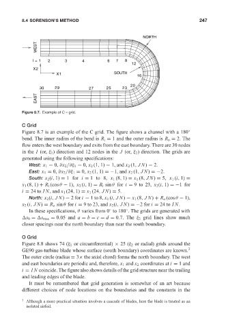
Figure 8.7. Example of C – grid.

C Grid
Figure 8.7 is an example of the C grid. The figure shows a channel with a 180 ◦
bend. The inner radius of the bend is R i = 1 and the outer radius is R o = 2. The
flow enters the west boundary and exits from the east boundary. There are 30 nodes
in the I (or, ξ 1 ) direction and 12 nodes in the J (or, ξ 2 ) direction. The grids are
generated using the following specifications:
West: x 1 = 0, ∂x 2 /∂ξ 1 = 0, x 2 (1, 1) = 1, and x 2 (1, JN) = 2.
East: x 1 = 0, ∂x 2 /∂ξ 1 = 0, x 2 (1, 1) =−1, and x 2 (1, JN) =−2.
South: x 2 (i, 1) = 1 for i = 1to8, x 1 (8, 1) = x 1 (8, JN) = 5, x 1 (i, 1) =
x 1 (8, 1) + R i (cos θ − 1), x 2 (i, 1) = R i sin θ for i = 9to23, x 2 (i, 1) =−1 for
i = 24 to IN, and x 1 (24, 1) = x 1 (24, JN) = 5.
North: x 2 (i, JN) = 2 for i = 1to8, x 1 (i, JN) = x 1 (8, JN) + R o (cos θ − 1),
x 2 (i, JN) = R o sin θ for i = 9 to 23, and x 2 (i, JN) =−2 for i = 24 to IN.
◦
In these specifications, θ varies from 0 to 180 . The grids are generated with
◦
s 0 = s max = 0.05 and a = b = c = d = 0.7. The ξ 2 grid lines show much
closer spacings near the north boundary than near the south boundary.

O Grid
Figure 8.8 shows 74 (ξ 1 or circumferential) × 25 (ξ 2 or radial) grids around the
GE90 gas-turbine blade whose surface (south boundary) coordinates are known. 3
The outer circle (radius = 3× the axial chord) forms the north boundary. The west
and east boundaries are periodic and, therefore, x 1 and x 2 coordinates at i = 1 and
i = IN coincide. The figure also shows details of the grid structure near the trailing
and leading edges of the blade.
It must be remembered that grid generation is somewhat of an art because
different choices of node locations on the boundaries and the constants in the

3 Although a more practical situation involves a cascade of blades, here the blade is treated as an
isolated airfoil.