Page 257 - Introduction to Computational Fluid Dynamics

P1: KsF/ICD
0 521 85326 5
May 10, 2005
16:28
0521853265c08
CB908/Date
236
Table 8.1: Solution to Equation 8.7. NUMERICAL GRID GENERATION
No. q (x) T

1 0 x
a
2 a x 1 − (1 − x)
2k
b 2
3 bx x 1 − (1 − x )
6k
b x
4 b (1 − x) x 1 − 1 − (3 − x)
3k 2
with boundary conditions T = 0at x = 0 and T = 1at x = 1. The solution to the
equation is
q q
x x 1 x
T =− dx dx + 1 + dx dx x. (8.7)
k k
0 0 0 0
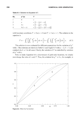
This solution is now evaluated for different assumptions for the variation of q
with x. The solutions are shown in Table 8.1 and Figure 8.3 with a = 2, b = 3, and
conductivity k = 1 in all cases. Clearly, the variation of T is controlled by variation

of q with x.
Now, to make Equation 8.6 a determinant of grid node locations, we simply
interchange the roles of x and T . Thus, the solution for q = bx, for example, is

1.0

0.8 4

2

0.6 1

T
3
0.4

0.2

0.0
0.00 0.25 0.50 X 0.75 1.00
Figure 8.3. Effect of q (x) function.