Page 256 - Introduction to Computational Fluid Dynamics

P1: KsF/ICD
CB908/Date
0 521 85326 5
0521853265c08
8.3 DIFFERENTIAL GRID GENERATION

Ro May 10, 2005 16:28 235

Ri
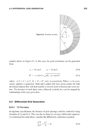
Figure 8.2. Eccentric annulus.
Θ ε

∗
R

annulus shown in Figure 8.2. In this case, the grid coordinates can be generated
from

x 1 = R cos θ, x 2 = R sin θ, (8.4)

%
∗ 2 2
R =− sin θ + R − ( cos θ) , (8.5)
0
where −π/2 ≤ θ ≤ π/2, R i ≤ R ≤ R , and is eccentricity. When = 0, a con-
∗
centric annulus is generated. Shah and London [66] have given results for fully
developed laminar flow and heat transfer in several ducts of noncircular cross sec-
tion. The domains of such ducts (sine, ellipsoid, cordoid, etc.) can be mapped by
relationships of the type given here.

8.3 Differential Grid Generation

8.3.1 1D Domains
In algebraic specification, the fineness of grid spacings could be controlled using
formulas (8.2) and (8.3). This can also be done by solving a differential equation.
To understand the main ideas, consider the differential conduction equation

2
d T q
+ = 0, (8.6)
dx 2 k