Page 206 - Introduction to Mineral Exploration

9: MINERAL EXPLORATION DATA 189

55,000

50,000

45,000

250,000 255,000 260,000 265,000 270,000 275,000 280,000

10
km Prospect
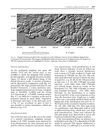
FIG. 9.6 Digital elevation model of the area based on the Ordnance Survey of Great Britain digital data
collected at 50 m intervals. The image is hillshaded with sun elevation of 45 degrees from 315 degrees so
SW–NE striking structures are highlighted. (Source: Digimap, University of Edinburgh.)

Remote sensing data tion spectrometry. Gold geochemistry is the
most obvious indicator of area for follow-up.
As the geological mapping was quite old Gold show a strongly skewed distribution
(Ussher 1912) and the oucrop poor, it was with a mean of 273 ppb, median of 10 ppb, and
possible to check the mapping with Landsat, maximum of 5700 ppb Au (Fig. 9.8). The soft-
air photography, and digital elevation models. ware used offers four options to divide the data:
Figure 9.6 shows a hill shaded image of the (i) quantiles – e.g. 20, 40, 60, 80, 100 percentiles
digital elevation model. A number of features in this case 5, 5, 24, 200, 5700 ppb; (ii) equal
can be detected by comparison with Fig. 9.3, intervals – 1140, 2280, 3420, 4560, 5700 ppb;
particularly the high ground underlain by the (iii) natural breaks (based on breaks in the
Staddon Formation, a coarse sandstone unit. histogram) 215, 708, 1540, 3100 ppb; (iv) mean
Some mapped structures are obvious, a mapped and standard deviations – 273, 1060, 1846,
fault at 266,000E, 51,000N and the strong 2633 ppb. As the distribution is so highly
N–S lineament at ~274,000E. Landsat images skewed and 40% of the concentrations are less
(Fig. 9.7) are difficult to interpret as the area is than the detection limit 10 ppb (set to 5 ppb),
intensely farmed in small fields. Vegetation in this case a percentile method based on the
is dominant and many of the dark gray areas higher part of the distribution was used: 50, 75,
of Fig. 9.7 are woodland. In spite of this it 90, 95 percentiles rounded to familiar numbers,
was possible to extract lineaments, which are 10, 150, 500, 1500 (Fig. 9.8). This map picks
shown in Fig. 9.10. out catchments with detectable gold as well
as differentiating those which have very high
Geochemical data gold concentrations. These were followed up
and gold grains were discovered in soil at the
One of the key data sets in the area is the result locations marked by the prospect symbols.
of a panned concentrate sampling exercise If the log-transformed data are plotted on a
(Leake et al. 1992). Samples were analyzed by probability scale (Fig. 9.9), a threshold of 50 pbb
X-ray fluorescence for trace elements and for might be selected. This simple subdivision is
gold by solvent extraction and atomic absorp- shown in Fig. 9.9, although it is, at least in the