Page 208 - Introduction to Mineral Exploration

9: MINERAL EXPLORATION DATA 191

55,000

50,000

45,000
5
km
N
250,000 255,000 260,000 265,000 270,000 275,000 280,000

3.59
2
Legend
Prospect log 10 2.26 1
Au (ppb)
River .93
0
Au ppb
–.4 –1
0.5–50
–1.74 –2
50–5700
0 10 30 50 70 90 98
percentiles (probability scale)

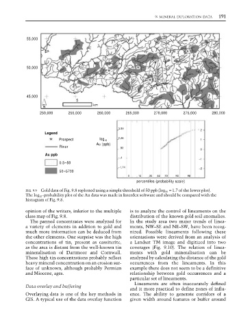
FIG. 9.9 Gold data of Fig. 9.8 replotted using a simple threshold of 50 ppb (log 10 = 1.7 of the lower plot).
The log 10 –probability plot of the Au data was made in Interdex software and should be compared with the
histogram of Fig. 9.8.

opinion of the writers, inferior to the multiple is to analyze the control of lineaments on the
class map of Fig. 9.8. distribution of the known gold soil anomalies.
The panned concentrates were analyzed for In the study area two major trends of linea-
a variety of elements in addition to gold and ments, NW–SE and NE–SW, have been recog-
much more information can be deduced from nized. Possible lineaments following these
the other elements. One surprise was the high orientations were derived from an analysis of
concentrations of tin, present as cassiterite, a Landsat TM image and digitized into two
as the area is distant from the well-known tin coverages (Fig. 9.10). The relation of linea-
mineralisation of Dartmoor and Cornwall. ments with gold mineralisation can be
These high tin concentrations probably reflect analyzed by calculating the distance of the gold
heavy mineral concentration on an erosion sur- occurrences from the lineaments. In this
face of unknown, although probably Permian example there does not seem to be a definitive
and Miocene, ages. relationship between gold occurrences and a
particular set of lineaments.
Lineaments are often inaccurately defined
Data overlay and buffering
and it more practical to define zones of influ-
Overlaying data is one of the key methods in ence. The ability to generate corridors of a
GIS. A typical use of the data overlay function given width around features or buffer around