Page 266 - Introduction to Petroleum Engineering

DECLINE CURVE ANALYSIS 253

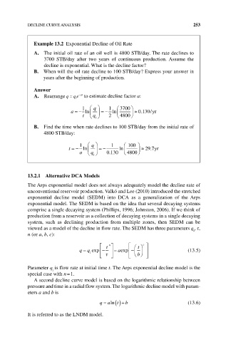
Example 13.2 Exponential Decline of Oil Rate
A. The initial oil rate of an oil well is 4800 STB/day. The rate declines to
3700 STB/day after two years of continuous production. Assume the
decline is exponential. What is the decline factor?
B. When will the oil rate decline to 100 STB/day? Express your answer in
years after the beginning of production.

Answer
A. Rearrange q qe to estimate decline factor a:
at
i
1 q 1 3700
a ln ln 0 130/yr
.
t q 2 4800
i
B. Find the time when rate declines to 100 STB/day from the initial rate of
4800 STB/day:

1 q 1 100
t ln ln 29 7yr
.
.
a q 0 130 4800
i
13.2.1 Alternative DCA Models
The Arps exponential model does not always adequately model the decline rate of
unconventional reservoir production. Valkó and Lee (2010) introduced the stretched
exponential decline model (SEDM) into DCA as a generalization of the Arps
exponential model. The SEDM is based on the idea that several decaying systems
comprise a single decaying system (Phillips, 1996; Johnston, 2006). If we think of
production from a reservoir as a collection of decaying systems in a single decaying
system, such as declining production from multiple zones, then SEDM can be
viewed as a model of the decline in flow rate. The SEDM has three parameters q , τ,
i
n (or a, b, c):
t n t c
q q exp aexp (13.5)
i
b
Parameter q is flow rate at initial time t. The Arps exponential decline model is the
i
special case with n = 1.
A second decline curve model is based on the logarithmic relationship between
pressure and time in a radial flow system. The logarithmic decline model with param-
eters a and b is

q aln t b (13.6)
It is referred to as the LNDM model.