Page 267 - Introduction to Petroleum Engineering

254 PRODUCTION PERFORMANCE

Example 13.3 SEDM Model of Shale Gas Decline
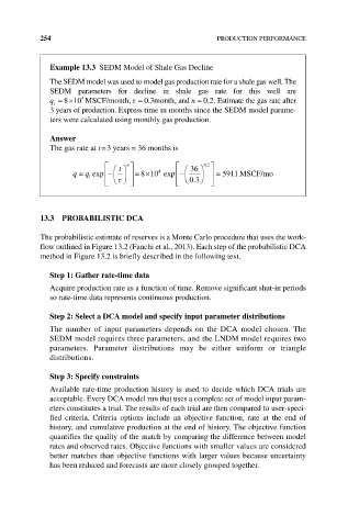
The SEDM model was used to model gas production rate for a shale gas well. The
SEDM parameters for decline in shale gas rate for this well are
.
q i 810 4 MSCF/month, 03.month, and n 02. Estimate the gas rate after
3 years of production. Express time in months since the SEDM model parame-
ters were calculated using monthly gas production.

Answer
The gas rate at t = 3 years = 36 months is

t n 36 . 02
q q exp 810 4 exp 5 5911 MSCF/mo
i
. 03

13.3 PROBABILISTIC DCA

The probabilistic estimate of reserves is a Monte Carlo procedure that uses the work-
flow outlined in Figure 13.2 (Fanchi et al., 2013). Each step of the probabilistic DCA
method in Figure 13.2 is briefly described in the following text.

Step 1: gather rate‐time data
Acquire production rate as a function of time. Remove significant shut‐in periods
so rate‐time data represents continuous production.

Step 2: Select a DCA model and specify input parameter distributions
The number of input parameters depends on the DCA model chosen. The
SEDM model requires three parameters, and the LNDM model requires two
parameters. Parameter distributions may be either uniform or triangle
distributions.

Step 3: Specify constraints
Available rate‐time production history is used to decide which DCA trials are
acceptable. Every DCA model run that uses a complete set of model input param-
eters constitutes a trial. The results of each trial are then compared to user‐speci-
fied criteria. Criteria options include an objective function, rate at the end of
history, and cumulative production at the end of history. The objective function
quantifies the quality of the match by comparing the difference between model
rates and observed rates. Objective functions with smaller values are considered
better matches than objective functions with larger values because uncertainty
has been reduced and forecasts are more closely grouped together.