Page 265 - Introduction to Petroleum Engineering

252 PRODUCTION PERFORMANCE
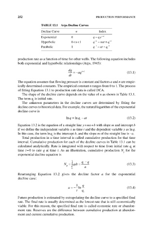
TABLE 13.1 Arps Decline Curves
Decline Curve n Index

Exponential 0 q qe at
i
Hyperbolic 0 < n < 1 q n nat q i n
Parabolic 1 q 1 at q i 1

production rate as a function of time for other wells. The following equation includes
both exponential and hyperbolic relationships (Arps, 1945):
dq aq n 1 (13.1)
dt
The equation assumes that flowing pressure is constant and factors a and n are empir-
ically determined constants. The empirical constant n ranges from 0 to 1. The process
of fitting Equation 13.1 to production rate data is called DCA.
The shape of the decline curve depends on the value of n as shown in Table 13.1.
The term q is initial rate.
i
The unknown parameters in the decline curves are determined by fitting the
decline curves to historical data. For example, the natural logarithm of the exponential
decline curve is

lnq lnq i at (13.2)
Equation 13.2 is the equation of a straight line y = mx + b with slope m and intercept b
if we define the independent variable x as time t and the dependent variable y as ln q.
In this case, the term ln q is the intercept b, and the slope m of the straight line is –a.
i
Total production in a time interval is called cumulative production for that time
interval. Cumulative production for each of the decline curves in Table 13.1 can be
calculated analytically. Rate is integrated with respect to time from initial rate q at
i
time t = 0 to rate q at time t. As an illustration, cumulative production N for the
p
exponential decline equation is
t q q
N p qdt i (13.3)
0 a

Rearranging Equation 13.2 gives the decline factor a for the exponential
decline case:

1 q
a ln (13.4)
t q i
Future production is estimated by extrapolating the decline curve to a specified final
rate. The final rate is usually determined as the lowest rate that is still economically
viable. For this reason, the specified final rate is called economic rate or abandon-
ment rate. Reserves are the difference between cumulative production at abandon-
ment and current cumulative production.