
Page 182 - MATLAB an introduction with applications
P. 182
Control Systems ——— 167
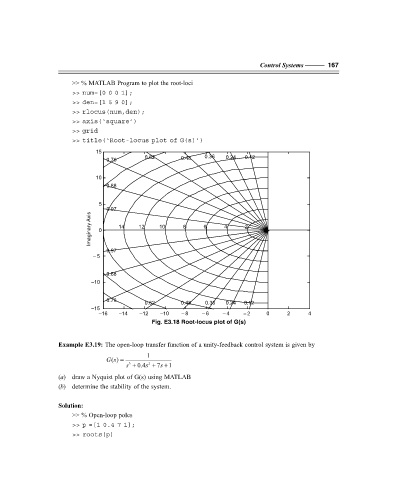
>> % MATLAB Program to plot the root-loci
>> num=[0 0 0 1];
>> den=[1 5 9 0];
>> rlocus(num,den);
>> axis(‘square’)
>> grid
>> title(‘Root-locus plot of G(s)’)
15
0.62 0.48 0.36 0.24 0.12
0.76
10
0.88
5
0.97
Imaginary Axis 0 14 12 10 8 6 4 2
0.97
–5
0.88
–10
0.76
0.62 0.48 0.36 0.24 0.12
–15
–16 –14 –12 –10 –8 –6 –4 –2 0 2 4
Fig. E3.18 Root-locus plot of G(s)
Example E3.19: The open-loop transfer function of a unity-feedback control system is given by
1
() =
Gs
s + 0.4s + 7s + 1
3
2
(a) draw a Nyquist plot of G(s) using MATLAB
(b) determine the stability of the system.
Solution:
>> % Open-loop poles
>> p =[1 0.4 7 1];
>> roots(p)
F:\Final Book\Sanjay\IIIrd Printout\Dt. 10-03-09