Page 184 - MATLAB an introduction with applications

Control Systems ——— 169

2
+ K s ( + 2 s+ ) 5
R(s) C(s)
2
s ( s + 3 )( s+ 5 )( s + s 5 . 1 + ) 1
–
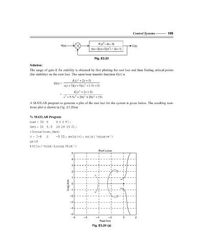
Fig. E3.20
Solution:
The range of gain K for stability is obtained by first plotting the root loci and then finding critical points
(for stability) on the root loci. The open-loop transfer function G(s) is

Ks + 2s + 5)
2
(
G(s) =
( ss + 3)(s + 5)(s + 1.5s + 1)
2
Ks + 2s + 5)
2
(
=
2
3
5
4
s + 9.5s + 28s + 20s + 15s
A MATLAB program to generate a plot of the root loci for the system is given below. The resulting root-
locus plot is shown in Fig. E3.20(a).
% MATLAB Program
num = [0 0 0 1 2 5];
den = [1 9.5 28 20 15 0];
rlocus(num,den)
v = [–8 2 –5 5]; axis(v); axis(‘square’)
grid
title(‘Root-Locus Plot’)
Root Locus
5

4
3
2
x
1 x
Imag Axis 0 x x

–1
x
–2

–3
–4
–5
– 8 – 6 – 4 – 2 0 2
Real Axis
Fig. E3.20 (a)

F:\Final Book\Sanjay\IIIrd Printout\Dt. 10-03-09